Experiences
Our Computing and Quantitative modeling experience comes from a variety of sources. Below we list some of the computing activities.
1. Learning with Incomplete Data using Neural Network

Estimation with incomplete data is very common in practical domains. EM algorithm, is one of the best tools in this regard. EM algorithm is an iterative algorithm where in each iteration a maximum likelihood regression is used. But, in some problems of practical importance (like predicting rare volatility surface patches in computational finance), a variable with more frequent misses in its values is considered to have less reliability in its available values than others. For example, a variable with 50% miss of values is less reliable data than a variable with 30% miss in its values. In this type of situations, a learner which can learn considering this reliability factor will perform better than the EM algorithm. So, we designed a learner, using feed-forward neural network, which can modify its learning rate for each observation upon considering the reliability factors of the observation's variables.
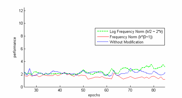 Figure:Performance of Learner with different weighting factors for learning rate
PowerPoint Presentation: ANN-Missing-Data.pps
Document for Full Procedure : ANN-vol-surf.pdf
2. Shock Detection in Stock Market Top

Stock market index is a measure of stock market's status. Volatility represents its uncertainty. Whenever an event occurs that deteriorates the market condition, the volatility suffers a sharp change. Some changes occur, even when there are no noticeable intervening shocking events in the market. So, its hard to say that a shock has occurred only seeing the sharp changes in volatility curve. Keeping this in consideration, some sophisticated techniques are inevitable to introduce. In this project, our effort was focused on giving a viable and realistic approach that can be used to detect the shocks in a stock market.
Implementation Details
The front end of the implementation was built using C# and backend using MATLAB. The implementation assumes that we are given price index of stock markets for a user specified time period. The series of data is considered as a time series. At first we calculate the volatility using appropriate technique. Next, we discretize the time series, clusterize nearby shock hosting candidates, and calculate Relative Volatility using the formula: (CT represents Central Tendency. e.g., median)

Next, the top 2 percentile (or N percentile)are taken as the Shock hosting dates.
Experimental Findings
The experimental result shows much similarity with the historical dates of shock occurrences. The possible shocks are marked with dark red dots:
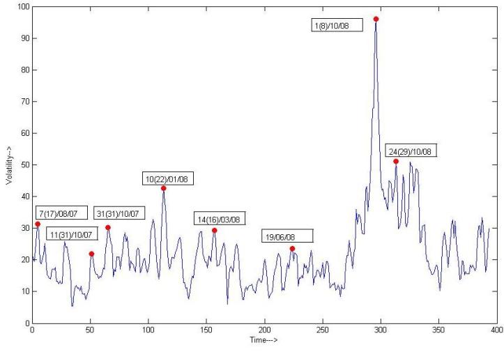
The events that occurred in the detected shock days are shown in the following table:
| Date | Reasons |
| August 2007 (1st dot) | During the week of August 6, 2007, a number of quantitative long/short equity hedge funds experienced unprecedented losses |
| October 2007 (3rd dot) | Huge change in Dow Jones Industrial Index |
| January 2008 (4th dot) | Oil price surpasses $100 per barrel |
| March 2008 (5th dot) | Bean Stearns Companies, Inc was sold to JP Morgan |
| October 2008 (7th and 8th dot) | Large losses in financial market worldwide |
PowerPoint Presentation: Shock Detection.pps
3. Lead-Lag structure between two time series Top

Determination of lead-lag structure between two time series is of utmost importance because with the help of it we can infer market dependency. Determination of lead-lag structure between two time series is a challenging task. The problem becomes more complicated because we are considering financial data. The principal challenges are:
- Varying lengths of lead and lag
- Shape invariance
Implementation Details
The methodology used for solving the problem was based on Dynamic Programming. We are given two time series, X(t) and Y(t), where t = 1,2,...,N. We compute the Distance Value of X(i) and Y(j), by the formula:

Next, E(i, j), which represents the optimal path weight to a point (i, j) is computed by the following formula:

Once the E(i, j) value is computed for each point (i, j), The optimal path is backtracked and constructed starting from the node with lowest E(I, j). The predecessor record is used to track the path backward. The path represents the optimal lead-lag structure. We used Matlab for building the back end and C# for building the front end.
Experimental Findings
In the path that was constructed using the above steps, every (i, j)th entry denotes the maximum dependency between two days in two time series. Last j value is considered counterpart for i. (j - i) values are plotted against i. If this value is positive, it says that the time series indexed by I is lead by the time series indexed by j and vice versa. To give the optimal lead-lag structure a realistic view, we limited the length of the lead or lag to a specified time difference. This is natural since a shock is unlikely to affect another market after a long time.
Now, lets come to some graphical depiction of the algorithm's performance. In the following, there are 2 figures. In both these figures, the first subplot represents the volatility of S&P data of USA, and the second graph shows the volatility graph of Indian S&P CNX 500 data. The third graph shows the optimal lead-lag relation of these two time series, as computed by the algorithm. For the first figure, the 3rd subplot employs a 60 day threshold and in the 2nd figure, the 3rd subplot employs a 400 day threshold.
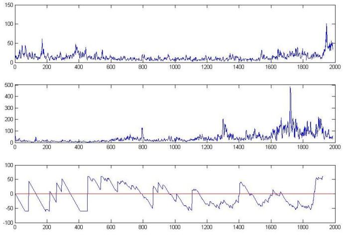
Figure 1: Result using 60 day threshold
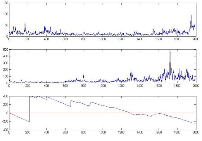
Figure 2: Result using 400 day threshold
4. Visualization of 4 dimensional data in a 2 dimensional spaceTop
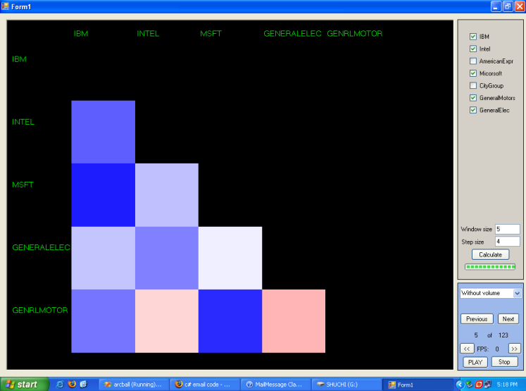
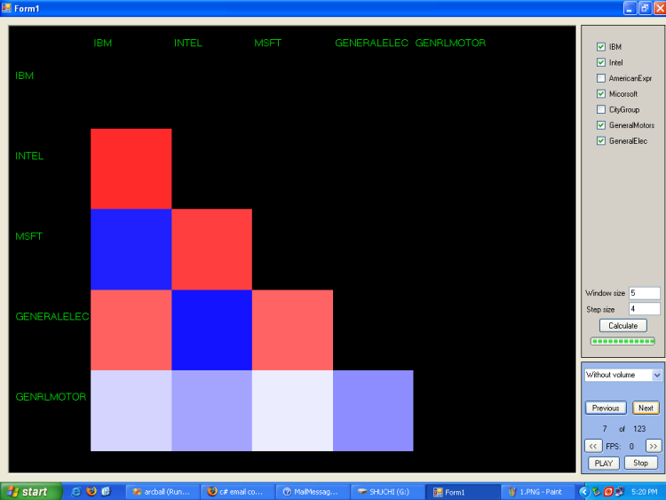
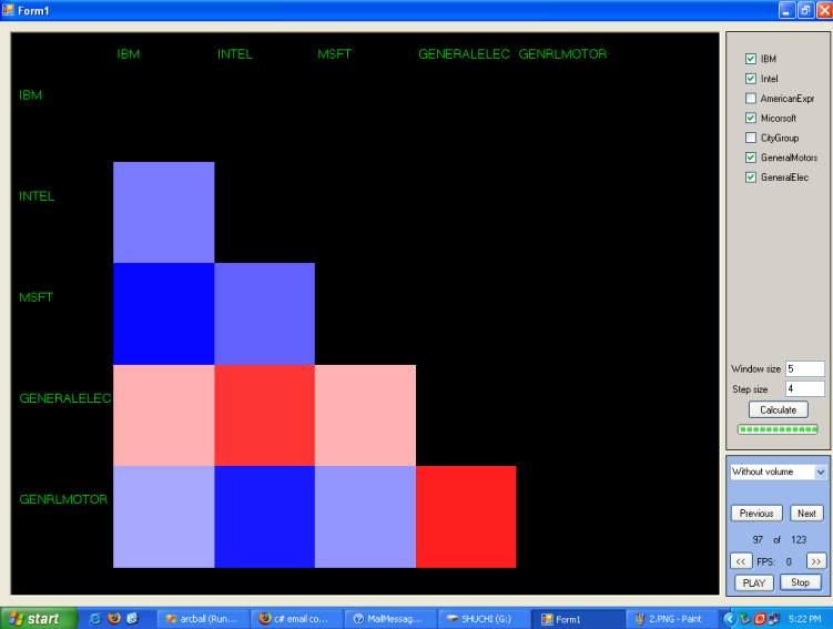
Visualization of higher dimensional data is very common in the field of Information Visualization. This project is to visualize 4 dimensional data in 2D space. Here, the regions (or points) of XY plane is used to represent 2 dimensions and color on the surface is used to represent another dimension. Time, which happens to be last dimension (and forth), is implemented by using a play button; i.e., after pressing the play button, colors of different patches of the surface change with time (please, see the video below)
Implementation Details
Stochastic Logic, ACI, there is a comprehensive data repository: like open share prices of big companies (e.g., Microsoft, IBM, Intel, General Motors, General Electronics, Citigroup etc.) for the past 5 years or so. To gain the interdependency between companies, we wanted to calculate co-variance (a 2D Matrix) of "open prices" of different companies as time series; i.e., first covariance was calculated within a specific time window (e.g., between 15-January-2007 to 30-January-2007), and then the next covariance's time window was taken after a specific time gap (e.g., next time windows can be say, after 10 days between 25-January-2007 to 5-february-2007). So, the problem can be alternatively said an moving window covariance matrix visualization.
| Variables | Dimensions used |
| Covariance Matrix | Requires two dimension |
| Covariance between two companies |
Color Coded between, where a value of -1 gets full RED, a value of 1 gets pure BLUE,
and 0 gets a value of WHITE (N.B. value of covariance between two companies is between [-1,1]). |
| Time | A PLAY button is used to show covariance matrices at increasing times |
Here covariance matrices are symmetric matrices and has diagonal elements equal to 1. So, we have shown only the lower triangle of covariance matrices. For this project Visual C# 2005, Visual C++ 6, S-plus, MATLAB, OpenGL, Microsoft Excel were used.
Description of Figures
In the following, three images depict covariance matrices at different time steps. Also, a video is added to show how the program depicts information as a movie of covariance metrics where each frame carries information of covariance matrices at different times:
5. Forecasting and Structural analysis of Multivariate Time Series Top
In the domain of Financial Computation, it is very common that one company's share
price is correlated with the price of another company's share. For example, the
share price of Microsoft is strongly correlated with the share price of IBM. So,
to forecast the future price of a share of Microsoft, one should consider the price
of IBM's share. Also, in that sort of situation, a natural question arises that
"To what degree the share prices of Microsoft and IBM are dependent on each other?".
In this project, we have fitted several statistical models (VAR, ARMA, GARCH) to
understand and subsequently predict future share prices of Microsoft and IBM, using
historical price data of Microsoft and IBM. Structural analysis of share prices;
i.e., inter-dependency between share prices of Microsoft and IBM; was calculated
using Granger Causality.